Names in Formulas, Naming Cells and Group of Cells
Creating names for Cells and group of cells will simplify your life and
make your formulas much easier to understand and track.
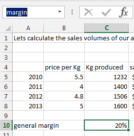
Here is what we want to achieve. For an apple farm we want to know the sales
amount and profit for each year.
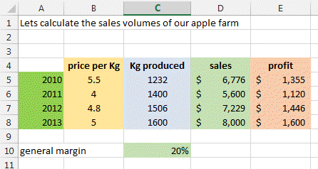
Here you have for the years 2010 to 2013 the amount of apples that were
produced and the price per kilogram.
The sales amount is the price per kilogram x the
amount of apples.
So lets name the various parts of the table.
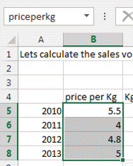
First select the cells B5 to B8 which include all the years prices. This is
the first range B5:B8.
And in the top left of the picture in the naming box, type the "priceperkg"
or PriceperLBS if you are using the imperial system.
Do the same for the number of apples.
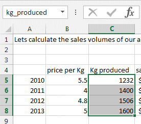
So now you have 2 ranges named. One is PriceperKg and the other is
Kg_produced.
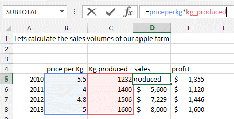
In the cell D5 type now the formula =priceperkg*kg_produced.
Press enter and drag or copy this cell to the bottom of your table.
This explained how to name a RANGE of cells.
Now lets calculate the margin.
The margin is sales price x margin.
Normally you would type in the profit cell something like this: =D5*$C$10.
The $ sign freeze the letter or number so that when you drag the formulas
referring to it, this frozen number or letter does not change.
With the naming, it is much easier and you can just name the cell C10 with
the name you want, like here "margin"
Lets add the margin formula in E5.
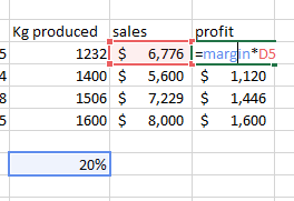
Lets write the profit formula in E5: =margin * D5. Then drag it down.
You see here I wrote D5 because the range for the sales is not defined
(yet). I
could also define it as sales and then the formula would be =margin*sales.
Name manager
The Naming Manager allows you to manage all the names you have created.
After
a while there can be many.
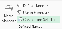
It is located in the FORMULAS Ribbon under Defined Names.
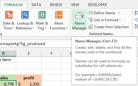
When you press on it the following window appears.
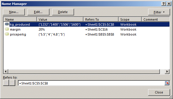
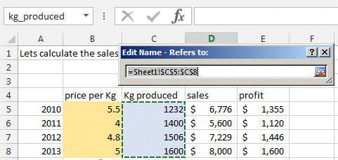
You can see the 3 names we have defined, with the value (or part of the
range), the coordinate of the range or cell and if this name is valid for
the full Workbook or just for the worksheet.
You can from there create new name, edit them and delete them.
So by double click on a name you will edit it and the following window will
open. This is the same window as the New name window.

So you can change the name, add comments and of course
change the range. If
you decide to click on the right side of the range line, on this small
button,  you will be sent to
the worksheet in order to select your cells.
you will be sent to
the worksheet in order to select your cells.
Create Name from Selection button
One easy way to create a name is by using the button Create from
selection
First select a range or a cell as well as the title (you must have a title
for your cell).
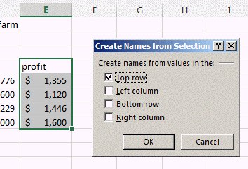
Excel will come with a suggestion, top, left, bottom, right but you are free
to change it.
Then select if it is in the top row or left column (which are the most used
cases) and press OK.
It will then automatically create the range with the selected name.
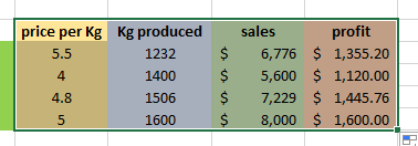
TIP: You can even create multiple names at once.
Example here: By selecting all the 4 columns, Excel will create
automatically the 4 names: price_per_Kg, Kg_produced, sales, profit !!!
Great time saving.
Write a formula easily
By using the button USE in FORMULA, you can easily type a formula.
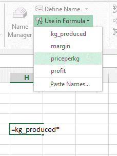
Here select the right name and click the name.

Now you should be much faster, and your spreadsheet will look great and be
very easily readable.
We hope it helped.
Please Tweet, Like or Share us if you enjoyed.
Download the sheet from
here.