Top 10 fonctions in Excel. The ones you MUST know.
Here are sumarized the number 6 to 10 most important functions and formulas that you need to have a good start with Excel.
Rank 6: Networkdays, workday, today()
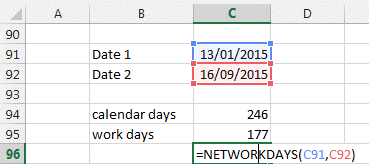
Getting the number of days between 2 dates is easy. Just Date1-Date2.
NETWORKDAYS(Date1, Date2) will remove all weekends and give you the real number of working days.

=Workday(start date, number of wordays) will give you the new date added with the "number of workdays".
Another formula is NETWORKDAYS.INTL, WORKDAY.INTL which lets you customize the weekends. You can have define weekends being only sundays, or saturdays, or even Monday & Tuesdays.
Rank 7: Max, Min, Large, Small, Rank
It is quite useful to be able to find the MINIMUM or MAXIMUM in a table.
Use MIN(range) or MAX(range) to find the Minimum or the Maximum in a range
To find the ranking of a number
=RANK(number, range, 1 for ascending order or 0 for descending order)
=SMALL(range,rank) : find the second small in a range =SMALL(range, 2)
=LARGE(range, rank)
Very useful for competitions and contests.
Rank 8: Text Formulas
Playing with words....is one of the great and funny side of Excel.
Check our Love Phrase Generator.
There are many ways to work with words. You can manipulate cells content with these main formulas
LEFT, RIGHT, MID: allows you to extract a portion of the text.
LEN: gives you the length of the text. Usually used together with LEFT, MID and RIGHT. LEN("I love Excel") gives 12
CONCATENATE or &: allows you to put text together.
SUBSTITUTE: Allows to replace some part of the text with some other.
TEXT: converts a cell into Text format and allows you to specify the format like here. =TEXT(3422332.6788,"#.0") becomes 3422332.7
FIND: allows you to find a chain of characters in a text. In "I love Chocolate" =FIND("Choco",B117) give 8, which is the position of the word Choco. You can then extract it with the MID function.
These are the main functions for text handling.
Do not forget to try our Love Phrase Generator.
Rank 9: IFERROR
In order to give a more professional feeling to your sheet and get rid of these errors messages that Excel displays (#DIV/0!, #N/A, #NAME?, #NULL!, #NUM!, #REF!, and #VALUE!), use the IFERROR function.
Find all about it here.
Rank 10: Combine MATCH, INDEX: ultimate power in Search
By combining both functions you get a perfect search function without the limitations of VLookup or Hlookup function.
You can search in any column or row and in any order.
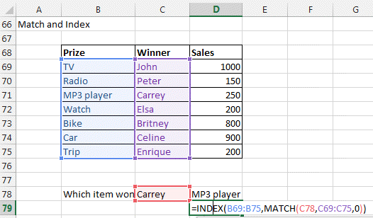
In our case

=INDEX(prize, MATCH(C78, winners, 0) )
=INDEX(list of values, MATCH(what you want to lookup, lookup column, 0))
For details about INDEX and MATCH go here.