Excel Made Easy

Get last 10 entries in a table in Excel

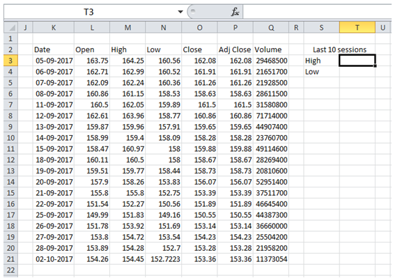
Table below is the raw data that I capture. I update one row for each trading day. I want to set up the Worksheet to automatically calculate the HIGH and LOW values for the last 10 sessions.

To do it in Excel, here is the answer:

a) High value in last 10 trading sessions corresponds to Max value among last 10 values in Col "High" (Col M).

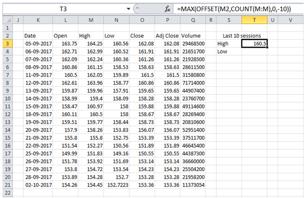
Enter formula =MAX(OFFSET(M2,COUNT(M:M),0,-10)) to get High value in last 10 trading sessions as shown below.

The first argument of OFFSET function refers to the Title in column as reference.

COUNT(M:M) counts numeric values in Column M (Title "High" is excluded since it is a text) and returns reference to the last cell with numeric value in Column M (M21)*** .

The fourth argument -10 extends the range referred by OFFSET by 10 rows above the last cell M21 to create the range M12:M21.

Max formula computes the maximum value in range M12:M21

***assuming no blank rows or rows with text in column M.

b) Low value in last 10 trading sessions corresponds to Min value among last 10 values in Col "Low" (Col N).

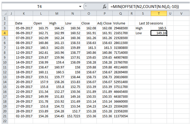
Enter formula =MIN(OFFSET(N2,COUNT(N:N),0,-10)) to get Low value in last 10 trading sessions as shown below.

The first argument of OFFSET function refers to the Title in column as reference.

COUNT(N:N) counts numeric values in Column N (Title "Low" is excluded since it is a text) and returns reference to the last cell with numeric value in Column N (N21)*** .

The fourth argument -10 extends the range referred by OFFSET by 10 rows above the last cell N21 to create the range N12:N21.

Min formula computes the maximum value in range N12:N21

***assuming no blank rows or rows with text in column N.

You can find similar Excel Questions and Answer hereunder

1) How can I get the most frequently occurring text in a range?

2) I have a large list of clients whose current Age I need to maintain in my database as it influences costs - how can I have Excel display the current age at all times?

3) How do you know which row was used the last. Here the explanation to find it with VBA

4) Can I add a small chart to Table data to make it visually appealing and easy to interpret?

5) How can I find the last used cell in a Column in VBA?

6) How can I declare a variable in VBA, what is important to declare

7) Is there a way to get a log value of a number using Excel?

8) How can I ensure that user enters only certain acceptable values in an input cell?

9) I conducted a test and the test scores are available - how can I get Percentile rank of students?

10) Filtering the value field in a pivot table in Excel