Alternate shade in data range in Excel
To do it in Excel, here is the answer:
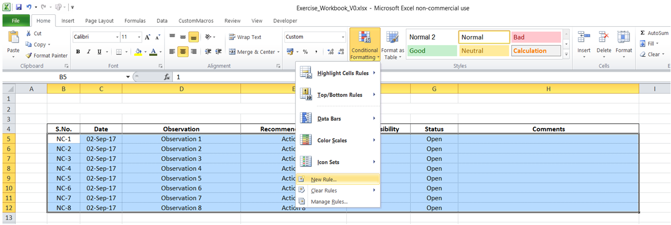
a) Select the data range where you would like to apply alternate row shading. Under "Home" tab, click on "Conditional Formatting" -> "New Rule".
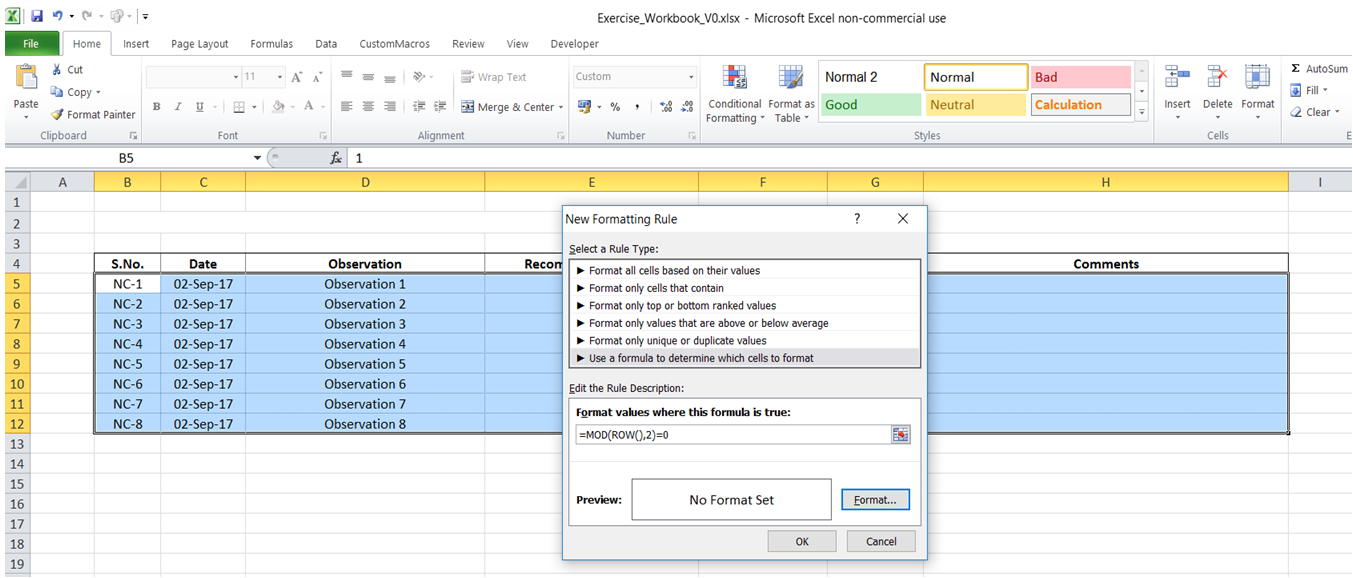
b) Select "Use a formula to determine which cells to format". Enter =MOD(ROW(),2)=0 in the "Format values where this formula is true" field.
The formula selects all even numbered rows. In case odd numbered rows need to be selected, change the formula to =MOD(ROW(),2)=1.
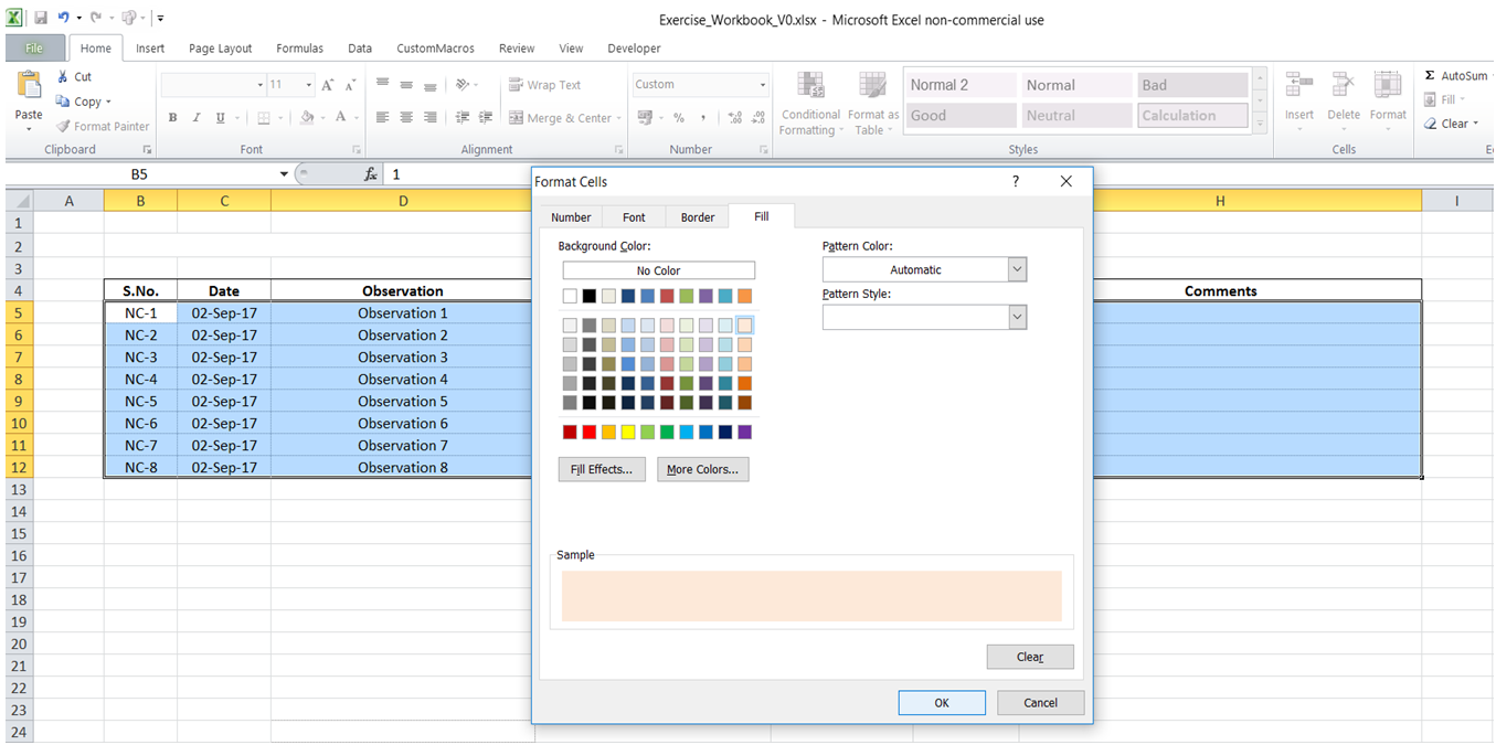
c) Click on Format-> Fill. Select color of your choice for shading. Click OK -> OK.
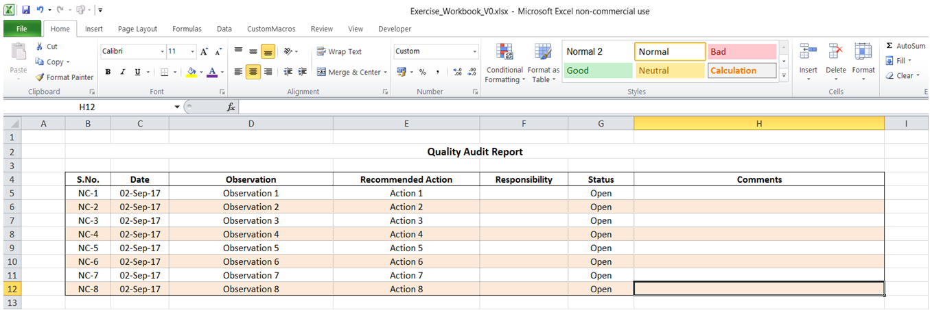
d) The selected range would be formatted as required with alternate rows shaded.
You can find similar Excel Questions and Answer hereunder
1) How can I set FreezePanes in a certain range using VBA?
2) How can I find the count of records that meet a given condition in my raw data table?
3) Is there a way I can average a range of numbers even if there is an error value in range?
4) How can I quickly remove all blank cells in a data range?
5) How can I use SUMPRODUCT to summarize my raw data?
6) How can I plot 2 series on the same chart with different scales / measurement unit for Values (Ex: Pareto chart)?
7) How can I find the count of records that meet multiple conditions in my raw data table?
8) Sumifs with date range as criteria in Excel
9) How to import xml data into Excel using VBA
10) How can I fill a series of data automatically?