Excel Made Easy

Conditional formatting visual stop lights in Excel

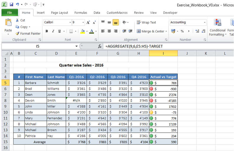
For example, if Target is met, there should be a Green light, if actual is closer to Target but not met, there should be a Yellow light and finally a Red light in case Actual is way off from Target.

In the dataset below, instead of looking at the Actual vs Target figures for each salesperson and then finding out if Target has been met, can there be lights automatically indicating performance of each salesperson?

To do it in Excel, here is the answer:

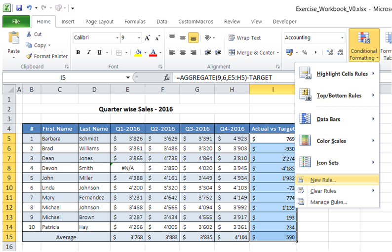
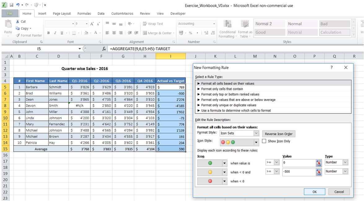
a) Select the data range with "Actual - Target" performance data. Under "Home" tab, click on "Conditional Formatting" -> "New Rule".

b) Select "Icon Sets" in the Format Style field.

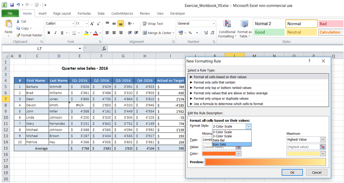
c) Enter the criteria for highlighting by selecting Type and value fields. In the example shown below, any value above 0 in the selected range will have Green light.

Similarly, any value between 0 and -500 will have yelow light and anything below -500 will have red light.

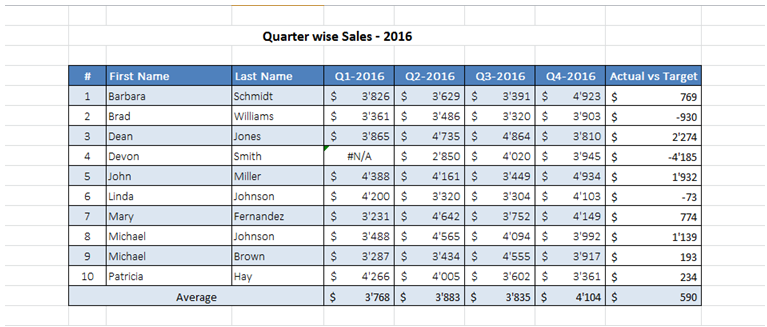
d) Click OK. The data range with "Actual - Target" performance data will appear as below.

You can find similar Excel Questions and Answer hereunder

1) I have a WorkBook that loads a form automatically when it is opened. In Excel, how can I suppress the form from loading on file open when required?

2) How can I get the last non-zero value in a row?

3) How can I find the slab in which a given value fits?

4) How can I prevent users from entering duplicate values in a range?

5) I am considering an investment of $500 per month for 3 years @ 6% interest rate. What is the Present Value of investment?

6) How do I know which cells on the worksheet contain Conditional Formatting?

7) How can I identify all cells with Conditional Formatting in my WorkSheet?

8) Is there a way to get a log value of a number using Excel?

9) Conditional formatting with if statement in Excel

10) How do I find the median salary of employees with the same skillset in my Organization?